August 29, 2016
Makeover Monday: U.S. Companies Are Hoarding Trillions Offshore

First, I must give credit for finding this week’s Makeover Monday to Jade Le Van. She’s a massive supporter of the work everyone has been doing in this project. Thank you Jade for finding this beauty from CNBC.
There are so many problems with this visualisation. However, the most egregious mistake is that the data is completely wrong. The author took the original data set, which has the total money held offshore by a company and allocated that same amount to every country that each country has an affiliate in. For example, General Electric has $199B stored in 18 offshore subsidiaries spread across seven countries. The author allocated $199B to EACH of those seven countries. That’s simply wrong!
What doesn’t work?
- The data is inaccurate.
- The pie charts are a ridiculous choice, especially when you show every single company in each country.
- The companies aren’t sorted.
- The size of the pies isn’t proportionate across the difference columns. In other words, they aren’t all based on the same range.
- It’s impossible to find a company you might be interested in investigating.
What works well?
- Nothing; the whole visualisation is a complete disaster.
I had a few minutes to explore this data set while on the bus home, so I opened up the data in Vizable. Within about 20 seconds I had two views that were far superior to the original.

Quickly and easily, I have a view of just how much money companies are keeping offshore and who they are in a nice, simple ranked list. Great! I already have something much better than the original.
Two more swipes in Vizable and I’m now looking at the companies with the most offshore subsidiaries.

At this point, I felt I basically had all I needed to tell the story in Tableau. I quickly reproduced the two charts from Vizable, then added a Pareto chart for more context. Lastly, I added some headers above each chart to tell a synchronous story.
April 25, 2016
Makeover Monday: Victims of the 21st-century Slave Trade

This week for Makeover Monday we are looking at this Viz of the Day from CNBC as seen on Tableau Public. For me, this is a really poorly done viz that really doesn’t tell us anything. When I look at this and say to myself “so what?”, I can’t answer that question.

Let’s start by looking at what works well:
- The table provides a nice summary of how many countries in each region fall into each tier.
- Clicking on a region and/or tier filters the map
- Nice “About” option
Really, that’s about all I can come up with that works well. There are so many things that could be done better:
- The most major problem is that there’s no context. What is good and what is bad? Is the situation getting better or worse? Context is so critical in visualisation and this viz totally lacks context.
- The title is misleading; was that intentional? These countries aren’t necessarily trafficking the children. Yes, it’s unbelieably terrible how the children are treated, but the title needs to be more accurate.
- The bubbles in the table add no value.
- Poor color choices
- Tooltips are useless
- There are no trends
- There’s no call to action. What am I supposed to do with this information? Again, so what?
Keep in mind that Makeover Monday is NOT about criticizing the author, it’s about critiquing the visualization and trying to create a more compelling story and more interesting visualizations.
What I wanted to try to focus on this week is whether or not childhood slave trade is getting better or worse. The data set that I created contains data back to 2007. Since we have geographical data (i.e., countries), I first wanted to see if viewing the countries by their tier status as a series of small multiple maps would reveal anything.
 |
| Click on the image to interact |
Unfortunately seeing trends across multiple maps is extremely difficult. Even if I drill into a specfic region, Africa for example, it’s still really hard to see patterns.
 |
| Click on the image to interact |
Ok, so maybe filtering even further by tier status would help. Let’s first look at all tier 3 countries.
 |
| Click on the image to interact |
Maybe you now have a case for making sense of the small multiple maps, but it takes too much work to see the rate of change. Enough of the maps, clearly they won’t work for displaying change. Fortunately Tableau lets us fail fast!
An alternative to the small multiple maps would be a heat map. In this view, I placed Country in the Rows and Year in the Columns and added a filter for Region.
 |
| Click on the image to interact |
Now we’re getting somewhere. I really like this view because it shows concentrations well. At a glance I can see that there were fewer Tier 2 in 2015 than in 2007 and more contries have moved towards Tier 3. It’s also clear that there are no more Tier 1 countries in Africa.
Contrast that to Europe.
 |
| Click on the image to interact |
Nearly every country in Europe is Tier 1 or Tier 2 and have been consistently. The transition in Russia from a Tier 2 Watch List to Tier 3 pops out as well.
So far, the heat map is my favourite. In Tableau though, since it’s so easy to create lots of views, I iterated some more. Next, I created this unit chart which shows each country in each region by year, simply color-coded by their tier status.
 |
| Click on the image to interact |
I love the look of this unit chart. Notice that I intentionally made each section 5 circles wide. I did that so they’re easier to count. Two things in particular jump out to me in this view:
- The number of Tier 2 Watch List and Tier 3 countries in Africa is growing.
- Asia had an increase in Tier 2 Watch List countries early on and is not slowly progressing more countries towards Tier 2 status.
To get an even better look at whether regions are progressing, I can filter the unit chart to only Tier 2 Watch List and Tier 3 countries. Filtering the data makes my two impressions above even more evident.
 |
| Click on the image to interact |
Lastly, I wanted to look at a time series view. In this case, I need to aggregate the data up to the Region level and count the number of countries in each Tier. The rationale behind this is to simply see how regions are doing over time. Are they getting better or worse? Is the number of Tier 1 and Tier 2 countries growing or are the number of Tier 2 Watch List and Tier 3 countries increasing?
 |
| Click on the image to interact |
It makes complete sense that the time-series view would reveal patterns best. That’s exactly the best use case for a line graph. I like the clean look about this chart. It’s easy to compare within a region and tier or across regions or across tiers or across regions and tiers.
But does this give me the BEST context? Is there a better way to show how the situation has changed since 2007? Yes, by comparing each year to the first year. In this view, I’m now showing the % change in the number of countries in each region in each tier since 2007. I’m using % change because it’s more contextual than simply the change.
 |
| Click on the image to interact |
In this post, I’ve shown you many ways to iterate through the data to find a compelling story, but this doesn’t bring it all together quite yet. In order to do so, I need to combine some of these views into a dashboard. I’m going long-form again this week as there’s simply too much information that needs to be shown to be effective in a single screen.
I’ve created both desktop and mobile version with the design a bit differnent in each.
October 5, 2015
Makeover Monday: Taxpayer in Some States are Voting with their Feet

Let’s start with the squared map.
- While some might see this as cute, it’s quite poor at communicating effectively. It’s difficult to compare the size of the squares. The size legend is essentially useless.
- The colour scale is not colour-blind friendly. I suppose he’s going for a stop light type of look, but that’s not even what this is because it has four colours, not three.
- The placement of the squares is not geographically accurate.
How about the scatter plot?
- Again, why the squares?
- Same colour issues as the map, but at least it’s consistent with the map.
- The annotations he added work well and the reference line at 50% aids in understanding, but both of those are merely encoding the same measure as the colour scheme.
- What is the scatter plot adding that the map is not already showing us?
And the line chart?
- This works well for a single state, but what if I want to compare states? What if I want to see all states at the same time so that I can see if there are any common themes?
- The colour scale is not consistent with the other two charts. Click on California and you’ll see what I mean.
One of the great things about Tableau Public is that most people allow you to download their workbooks so you can have a play for yourself. That’s exactly what I did in this case. I’ve build the dashboard below to address the communication issues that I feel the original has.
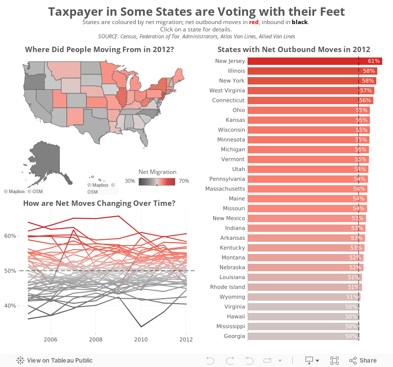
What did I do?
- Focused on a single metric, in this case net migration, since that’s what the original story was about.
- Used a single colour pallet that is colour-blind friendly
- Added all states to the line chart. Clicking on a state in the map will highlight the state on the line chart.
- Included a bar chart of the states that have a net outward migration
- Gave the visualisation a more meaningful title
What would you do differently? I’d love your suggestions for making this better.
October 20, 2014
Monday Makeover: Causes of Death in the USA

One of my frustrations with Viz of the Day, as I've noted on both of my appearances on the Tableau Wannabe Podcast, is that I suspect people look at these as examples of visualizations done well, even though that's not the true intent. Yes, I'm saying that anecdotally, but I base this off of a few conversations I've had with people about it.
In today's viz, there are an abundance of issues. Here are a few:
- The filled map makes it impossible to see the smaller states. In fact, it's nearly impossible to trigger the action when hovering over Rhode Island. Filled maps can easily skew the data towards the larger states, so a bubble map is preferred.
- The temperature diverging color palette for the map is not color-blind friendly.
- The colors on the map and on the packaged bubbles are too similar. Green on the map means a low rate, while green on the bubbles means cancer.
- The stacked bar chart in the middle adds no value. When you hover over a state, the packed bubbles changes, so what value is the stacked bar chart adding.
- Packed bubbles are a very poor way to communicate ranking. A sorted bar chart is better.
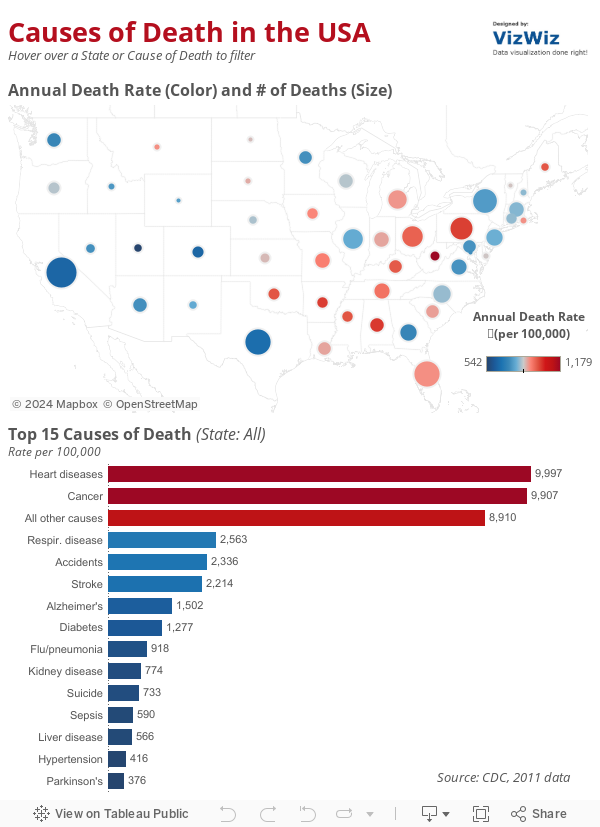
- I changed the map to a bubble map. Now it's easier to see all states because I've also sized the states by the number of deaths for additional context.
- I'm using a blue-red color palette consistently throughout to represent the death rate.
- I removed the individual colors for the diseases and colored them by the death rate instead.
- I killed the stacked bar chart. I also included an action from the bar chart to the map (in addition to the existing map to bar chart action).
- I changed the packed bubbles to a ranked bar chart.