June 28, 2017
Workout Wednesday: UK General Election Slopey Trellis Chart
election
,
level of detail
,
LOD calc
,
panel chart
,
politics
,
slope graph
,
small multiples
,
table calc
,
trellis chart
,
UK
,
united kingdom
,
Workout Wednesday
2 comments
That Emma! She's quite the sneaky stinker! For Workout Wednesday Week 26, she asked us to build a trellis chart full of slope charts that compares election results by political party by constituency for 2015 vs. 2017.Fortunately, I have my trellis chart calcs safely saved in my notes, so I didn't have to Google those. The tricky bit for me was the sorting. I'm not going to spoil how I did it for you, but you can download my workbook to see how I did it. As usual, Emma and I took very different approaches for the calculations required for the sorting. She used LODs for all of her calcs, I only used one. They both work though! It all depends on how your brain works I suppose.
The data prep parts were pretty straight forward (thank you Emma for alerting us to the need to do this). Emma loves little tricks in the formatting, but I didn't see any this week.
One thing I did different was to provide a "buffer" for the year labels. I place them 10% above the highest value so that they don't overlap the slope chart lines. Emma's year labels sometimes overlap with the slope chart lines. Just a personal preference for me.
Great fun Emma! Thanks! Took me about 90 minutes including this blog post on the train from Frankfurt to Hamburg. Great use of my time! #AlwaysLearning
Click on the image for the interactive version and to download.
June 26, 2017
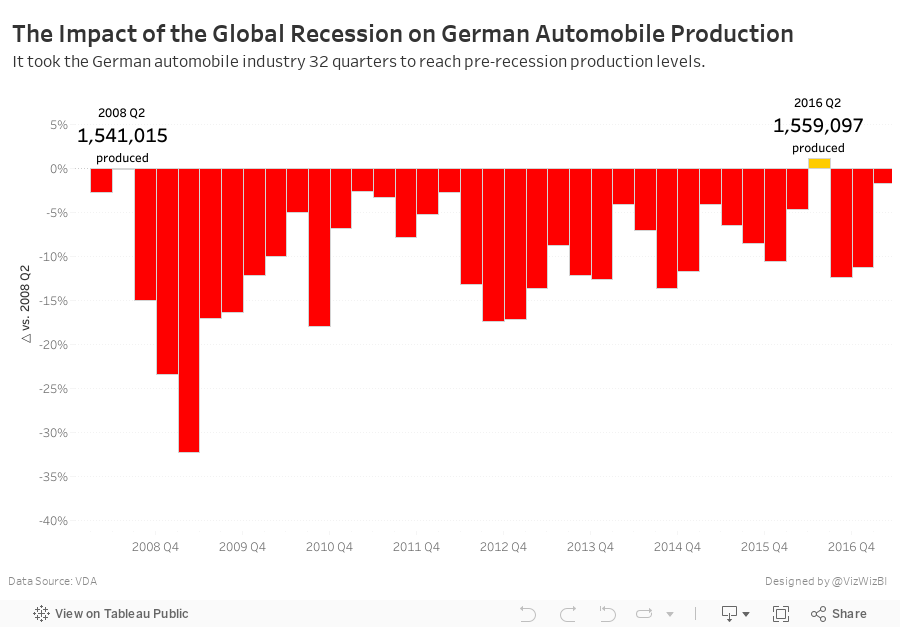
Makeover Monday: The Impact of the Global Recession on German Automobile Production
Life will be hectic these next two weeks. I'm off the Germany for 10 days, helping our German team with Zen Master events in Frankfurt and Hamburg before heading to Exasol Xperience in Berlin next week. This week, we're looking at German car production to make it more relevant for the #MakeoverMonday live sessions we'll be running.

What works well?
- Line charts are generally very easy to understand
- Including a trend line
- Great responsiveness for the tooltips
- Including the Year over Year change in the tooltip
- Including a BAN in the tooltip
- Putting the tooltip into a sentence
What could be improved?
- Needs a better title
- Remove the car icon from the tooltip
- Remove the up and down arrows from the tooltip; they're redundant to the text.
- It's pretty boring. What's the story?
What were my goals?
- Find a story in the data
- Create a more informative visualisation
- Explore the data, particularly with all the ways you can create time series in Tableau
- Keep the viz to a single worksheet in order to keep it simple
- Give the viz a meaningful title
- Use German colors
- Get it all done in an hour; I'm really pressed for time as I type this.
- Keep the idea of the tooltips from the original with the BANs.
Ok, that's it. Here's my Makeover Monday week 26 viz.
June 22, 2017
Makeover Monday: Tiled Heatmap of U.S. Air Quality Levels
air quality
,
AQI
,
heat map
,
Makeover Monday
,
Matt Chambers
,
ozone
,
tile map
,
tiles
,
United States
,
USA
No comments
I was very interested in looking at state-level air quality and built lots of heatmaps and originally built them in a single worksheet using table calcs to sort out which states go in which columns and rows.
This didn't work for me, though, because it only helped me see the states alphabetically. It's much more intuitive if they are displayed geographically. An idea popped into my head...
I wonder if I can combine a heatmap that looks at daily max reading by state across all years with a tile map.
I quickly went to Matt Chambers' great post for how build tile maps added the secondary data source, blended it by state and replaced my crazy table calcs with a simple tile map view. What a fun exercise! I learned a ton and feel like I created a much more intuitive view. Does anyone recall every seeing a tiled heat map? Have I come up with a new chart type???
Click on the image for the interactive version. Note that the viz might be slow to load as it's displaying about 460,000 marks.
June 21, 2017
Workout Wednesday: The Value of Top 3 & Top 5 Contributors
bar chart
,
cumulative
,
level of detail
,
LOD
,
percentage
,
running total
,
table calc
,
Workout Wednesday
2 comments
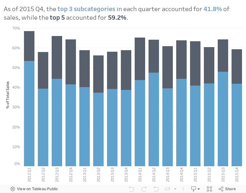
First, we wanted to understand what percentage of sales come from the top 3 and top 5 subcategories in each quarter, then we want to understand the cumulative contribution through time.
So that's your challenge. Build the viz below using this data source with these conditions:
- Match the title
- Match the tooltip
- Match the colors
- Show the contribution of the top 3 and the top 5 subcategories in each quarter
- Bar height represents the cumulative contributions from the first quarter
- Use only one worksheet
- Viz size is 800x600
I'm pretty sure that's everything. If I missed something, leave a comment or tweet me and I'll update the requirements. Remember to post you version to twitter and tag @EmmaWhyte and @VizWizBI. Good luck!
June 19, 2017
Makeover Monday: Is America Improving Its Ozone Air Quality?
actions
,
cycle plot
,
Data Duo
,
dot plot
,
EPA
,
Makeover Monday
,
ozone
,
pollution
,
sparkline
,
United States
,
USA
2 comments
The EPA website also contained some basic reporting, which is the focus for this week's makeover.
What works well?
- Simple layout. It's easy to see you have days within months going left to right and years going down.
- Colors match the official EPA colors for the AQI categories
- Including the ranges we know what constitutes a good reading vs. a bad reading
- The title tells me what I'm looking. Including the date range is a nice touch too.
- Using a strip plot along with the colors helps reveal seasonal patterns
- Including the source in the footer
What could be improved?
- Make the colors color-blind friendly
- It's difficult to see how a month has changed across the years.
- I can't hover to see the values.
- It says each “tile” represents one day of the year and is color-coded based on the AQI level for that day, but I think it's actually showing the max measurement for each day. It should be more clear what they are representing.
- There's very little context. How does one county compare to others? How does one county compare to the national average?
What were my goals?
- Last year I challenged The Data Duo to visualise an almost identical data set. Pooja created a pretty amazing viz (of course), so I wanted to pick some parts off of it. Particularly, the State selectors on each site and the dot plot.
- I wanted to understand how each month changed across the years, which is pretty much exactly what a cycle plot was created for. I used a trend line instead of an average though because that seemed to show the patterns better.
- I wanted to add context for comparisons to the national average and to the state average (which appears when you click on a state).
- I wanted to use color-blind friendly colors.
- I wanted a small sparkline-type chart to show how things have changed since 1990.
With these goals in mind, here is my Makeover Monday week 25 submission. Click on the image for the interactive version.
June 14, 2017
Workout Wednesday: Visualising the National Student Survey with Spine Charts
Emma was back at it again with her sneaky tricks for Workout Wednesday week 24. Read the requirements here. I'd never built a spine chart before so this was a fun challenge and great learning experience. I did do a few things differently than Emma though:- My main viz with the table and spine chart is all one worksheet. Emma chose to split it into two.
- My calculation for the % Agree is different than hers. She went with a straight average while I went with a weighted average.
- For one of the filters I used a data source filter while she used a context filter. Both work, just different approaches.
With that, here's my Workout Wednesday week 24. Click on it to see the interactive version.
June 13, 2017
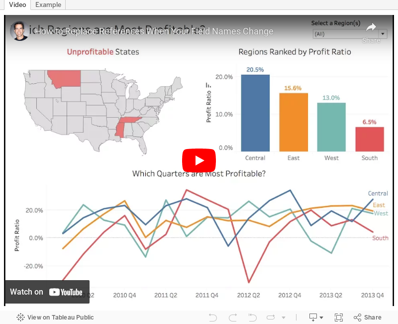
Tableau Tip Tuesday: How to Replace References When Your Field Names Change
In this example, I demonstrate what happens when the data source changes. You could also apply this method when you simply want to swap out all existences of one field for another. For example, you want to change all used of Order Date to Ship Date. Easy peasy!
You can also watch this directly on YouTube here if it doesn't render below.
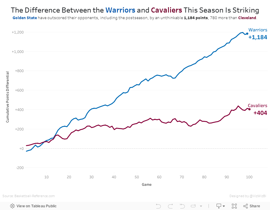
The Difference Between the Warriors and Cavaliers This Season Is Striking
basketball
,
Cleveland Cavaliers
,
color
,
comparison
,
context
,
cumulative
,
difference
,
Golden State Warriors
,
line chart
,
NBA
No comments
Last week I highlighted a really nice line chart from Business Insider over on my Data Viz Done Right site. As a learning exercise I wanted to recreate their chart while also incorporating the feedback I suggested. I highly recommend this process to anyone wanting to learn and practice; take a viz you like and try to rebuild it in Tableau.Since the Warriors won the NBA title last night, I've updated the viz with the latest data. Simple, fun, effective visualisation. And the Warriors are pretty damn good!
June 12, 2017
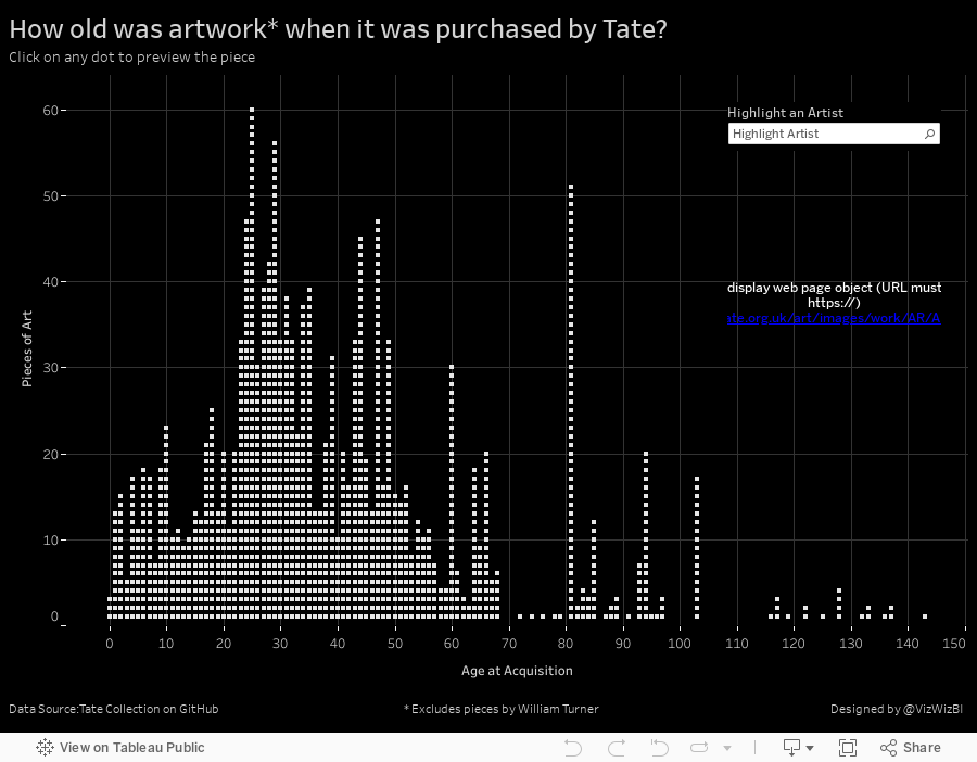
Makeover Monday: How old was artwork when it was purchased by Tate?
art
,
black and white
,
Makeover Monday
,
monochrome
,
Tate
,
unit chart
,
William Turner
No comments

What works well?
- A pie chart with two slices is really easy to understand.
- The slices are labeled so I don't have to guess at their values.
- The colors are easy to distinguish.
- The largest slice starts at 12 o'clock.
What could be improved?
- There's no title.
- Who is Turner? Why does he have such a large proportion?
- Is the data accurate? HINT: No, it doesn't match with the data on GitHub.
- There's no reference to the source.
- There's no really story to it. When I ask "so what?", I can't answer the question.
- It's boring.
What were my goals?
- Since Turner makes up 95% of the artwork, I'm more interested in everyone else. I've filtered out Turner.
- The Tate seemed to make purchased in bunches. Instead, how about looking at how old pieces are when they are purchased?
- What is the distribution of the age of the pieces purchased?
- Provide an option to find an artist.
- Include a way to view the piece of art as a thumbnail.
- Display every individual piece of art (inspired by Pooja Gandhi).
- Provide details in the tooltip.
- Make it look a bit more "artsy" by going with a monochrome theme.
Overall, this data set proved pretty challenging to find any insights. Turner was such a large proportion that I couldn't see anything in the data until I got rid of him. It also helped to hide all of the fields I didn't want to use. Two simple, yet effective ways to make the data more understandable.
June 11, 2017
Viva Las Vegans! An Iron Viz Entry
data.world
,
iron viz
,
Las Vegas
,
map
,
Tableau Conference
,
vegan
,
vegetarian
,
web data connector
No comments
This also gave me a chance to test the new web data connector from data.world. One of the data sets is a list of over 18,000 restaurants that serve vegetarian or vegan food in the US. I took this list, narrowed it down to Las Vegas, eliminated and closed restaurants and joined it to a Excel files that has the websites for each restaurant.
It's not anything too complicated nor flashy, but here's to hoping that practicality and usefulness is important to the judges as well. I've also designed it for mobile!
Enjoy!

June 7, 2017
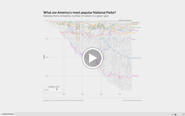
Workout Wednesday: National Parks Have Never Been More Popular
calculated field
,
fivethirtyeight
,
label
,
LOD
,
national parks
,
United States
,
USA
,
Workout Wednesday
No comments
- Dashboard must be 800x735
- Everything will need to be floated in the dashboard to make it look right
- Title, subtitle and viz must all be one worksheet
- Footers are separate with a line separating them from the viz
- Rank grid lines must be included at 1st, 25th, 50th and 75th. They must be labeled as I've done it.
- Year grid lines should only be shown for 1925, 1950, 1975, and 2000.
- Include an option for the viewer to pick a park to highlight
- When (None) is picked from the highlighter, then it should show the default view (first image below).
- When a park is selected from the highlighter, it should be the only line displayed and should be displayed as a black line (second image below) unless it's one of the default parks. In that case, it should retain its default color.
- Align the highlighter as I've done on the bottom left of the chart.
- Match the park names
- Match the tooltips (pay attention to the park names)
- Match the title and subtitle
- Match the line labels
- Viz and highlighter should be limited to National Parks and National Historical Parks
- OPTIONAL: Use the Raleway font
I suspect will probably find building the bump chart fairly straightforward. The tricky bits are the coloring, highlighter, park names, labels and grid lines. Feel free to ask questions if you get stuck.
Click on either image for the interactive version. I've also included a video demonstrating how the final viz should work.
Click on either image for the interactive version. I've also included a video demonstrating how the final viz should work.
Get the data here. Good luck!
June 5, 2017
Makeover Monday: America's Most Visited National Parks
area chart
,
bump chart
,
fivethirtyeight
,
Makeover Monday
,
national parks
,
pareto
,
popular
,
rank
,
small multiples
,
trends
,
United States
,
USA
5 comments
For week 23, we are looking at the popularity of America's National Parks. As an American, I've learned to cherish the amazing, free natural wonders sprinkled around the country. In particular, when we lived in California, we made it a point to visit Yosemite, Joshua Tree and the Grand Canyon amongst other places. They truly are worth a visit.
The viz that we are making over this week comes from FiveThirtyEight and it really quite fantastic, like most of their vizzes.

What works well?
- Great use of highlighting
- Including gridlines to help guide the eye
- Noting the source
- Nice use of a bump chart
- Shows patterns really well
- Subtitle explains how to interpret the viz
- Colors are distinct enough to follow through the viz
What could be improved?
- The title is very boring.
- Lack of interactivity
- How can I identify a park that's not highlighted? It would be nice to have a way to choose another park to highlight.
- The top 6 parks are highlighted, but why are the others highlighted? It seems pretty random.
- While this shows me the most popular parks, it lacks the context of how many visitors and how that has changed over the years.
What were my goals?
- Focus on the top 25 parks
- Focus on the last 50 years
- Include the visitors to provide more context when comparing parks
- Use a small multiples layout and try to recreate this viz that I highlighted on Data Viz Done Right
- Include the total visitors somewhere so the reader doesn't have to figure it out
- Create the entire viz in a single view (except the footers)
But then I had another question in my head: At State level data, how many States account for 80% of all visitors? For this, I created a simple Pareto chart. Two vizzes for the prices of one! Enjoy! Click on either image for the interactive version.
Subscribe to:
Posts
(
Atom
)


