May 28, 2019
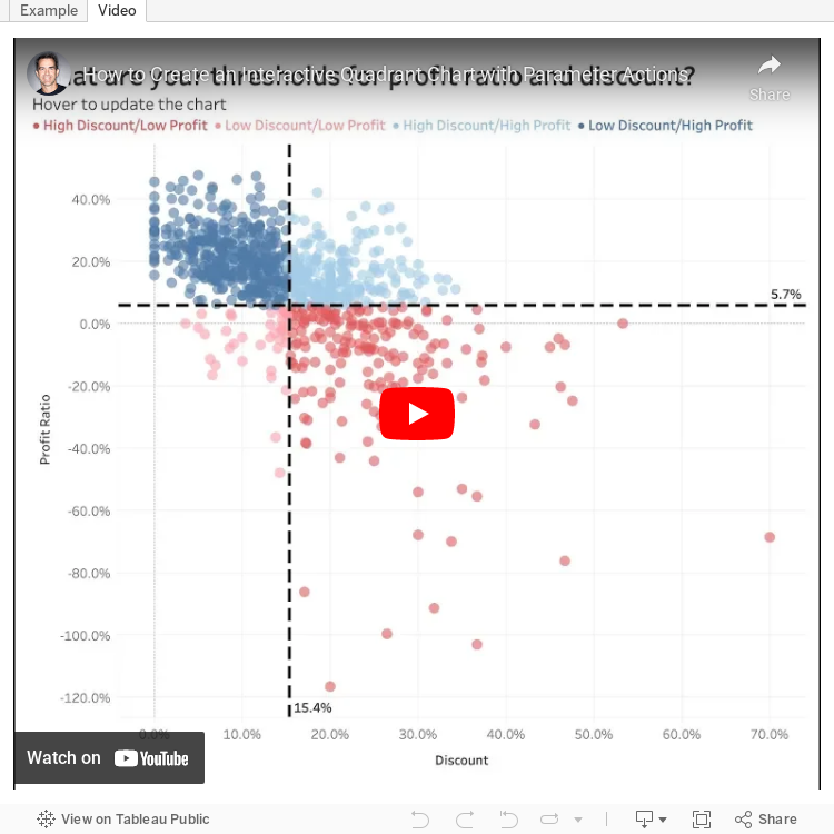
#TableauTipTuesday: Create an Interactive Quadrant Chart with Parameter Actions

The first chart I wanted to try was a quadrant chart. A quadrant chart colors each quadrant based on thresholds set for each axis in a scatter plot. Previously, I created two parameters and the user had to type in numbers to adjust the view. However, with parameter actions, I can now enable to use to update the quadrants by simply hovering over a dot.
And here's the video...enjoy!
May 27, 2019
#MakeoverMonday: What has happened since people started paying attention to climate change?
carbon dioxide
,
carbon footprint
,
climate change
,
co2
,
data studio
,
environment
,
Makeover Monday
,
pollution
,
world bank
No comments

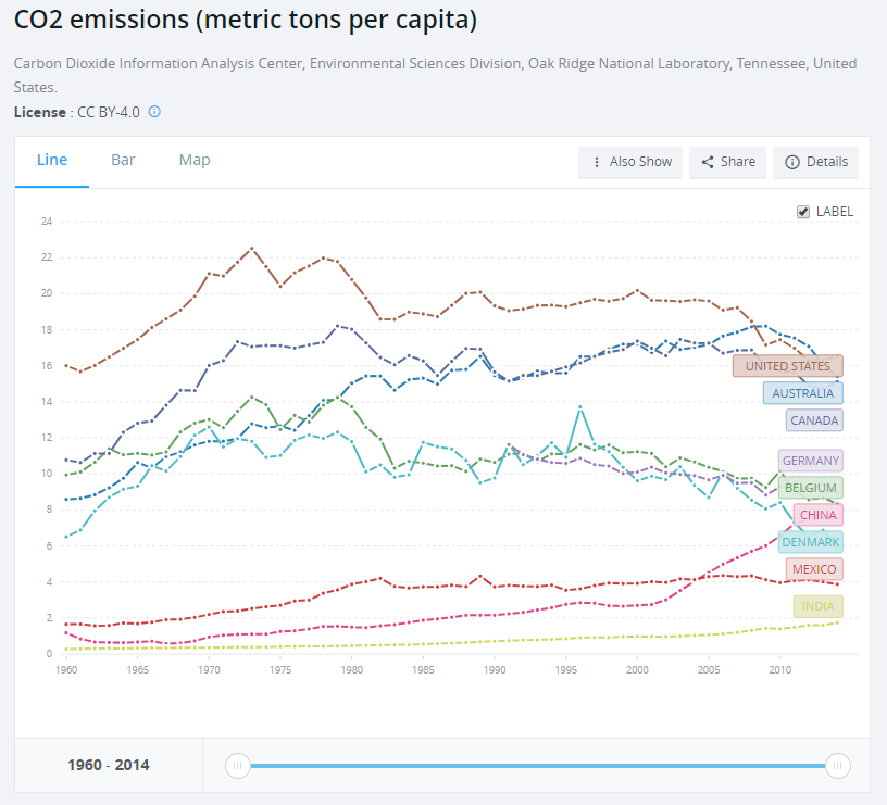
What works well?
- Using a line chart over time helps show the trends
- Including a slider filter for the user to zoom in on a specific period
What could be improved?
- Using dotted lines indicates there are breaks in the timeline, but there aren't. Therefore, a solid line should be used.
- The labels on the ends of the lines hide the data.
- It could use an impactful title and subtitle. Though I suppose this is just a report, not analysis.
What I did
I created a map to ensure that the country names were correct. When I did this, I then saw that there were lots of aggregations of countries. For some reason, the income level categories captured my attention so I filtered down to just those items.
The years 2015-2018 were include and didn't have any values. I filtered those out. There were years when no data was captured for some countries. I filtered those out.
I plotted the data as a line chart and created a calculation to show the change vs. the first year for each country. I noticed that there was a spike in CO₂ per capita in 1973 for high income countries. This reminded me of the oil crisis of 1973, but that wouldn't have anything to do with carbon emissions I wouldn't think.
That got me thinking about climate change in general. I entered "when did people start paying attention to climate change" into Google and the first search result was an article from National Geographic titled "Climate Change First Became News 30 Years Ago. Why Haven’t We Fixed It?"
This particular line was what I was looking for: "The Intergovernmental Panel on Climate Change was established in late 1988..."
So, back to the data I went and I filtered the data to 1988-2014 and compared every subsequent year to 1988 in order to see how much things have changed since climate change started garnering some attention. I expected high income countries to have ever increasing CO₂ per capita. I was wrong.
It turns out that the middle income countries have had the largest change in CO₂ per capita. So that became the focus of this analysis.
May 21, 2019
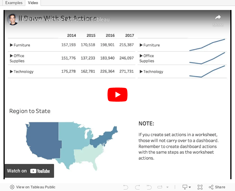
#TableauTipTuesday: Drill Down With Set Actions

Enjoy!
May 20, 2019
#MakeoverMonday: Bear Attacks in North America
animals
,
bar chart
,
bear
,
bears
,
Canada
,
Makeover Monday
,
north america
,
unit chart
,
United States
,
Vox
No comments

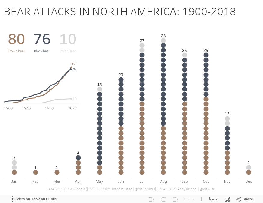
Vox has an interesting article and has the visualization that we'll makeover this week.

What works well?
- The title summarizes the findings.
- The sub-title provides context.
- Including the source and author's name
- Using a bar chart
- Including the numbers in the bars
- Including the gridlines to make the bars easier to compare
- Good use of color
What could be improved?
- The bear icons should be removed.
What I did
I really liked Hesham Eissa's viz this week, so I used that as inspiration for mine.
- His unit chart points downward, but I wanted mine to point upward.
- I like his BANs, so I included some of my own, but different numbers.
- I included the total for each month as he did.
- Hesham's dot are colored by the location (US vs. other), while I colored mine by the type of bear.
- I included a line chart to show the cumulative attacks by type of bear since 1900.
Thanks for the inspiration Hesham!!
May 16, 2019
The History of English Football Champions: 1888-2018
animation
,
champions
,
england
,
English Premier League
,
flourish
,
football
,
soccer
,
timeline
No comments

Given that this requires animation, I knew I needed a tool that supported this and I turned to Flourish. The data has to be structured in a very specific way, so I downloaded the data from Wikipedia, imported it into Alteryx for a bit of a massage, and spit it back out in the format Flourish required.1889 ➡️ 2̶0̶1̶8̶ 2019— Squawka Football (@Squawka) May 13, 2019
Watch the race to become the most successful club in English top-flight history unfold before you. Now updated. pic.twitter.com/4IprWQ16ZT
And voila! An animated viz of the history of English football champions from 1888-2018. Very little effort required + great animation = win!
May 13, 2019
#MakeoverMonday: Rhino poaching in South Africa - Is the decrease a real reversal?
animals
,
Makeover Monday
,
poaching
,
rhino
,
rhinoceros
,
South Africa
,
wildlife
,
WWF
No comments

This week's viz is a count of rhinos poached from 2006-2016.

WHAT WORKS WELL?
- The title and subtitle tell me what the viz is about.
- Using a single color
- The design clearly shows that there was a steady increase in rhinos poached over a 10 year period until the decline in 2016.
- Including the labels at the top of the unit chart for context.
WHAT COULD BE IMPROVED?
- What value does each rhino image represent? Whatever it is, it's not accurate as the same number of units represent different values.
- Is the rhino image necessary? I would try it without it.
WHAT I DID
- I read the source article for context and to give me ideas for my analysis.
- I changed the chart to a bar chart, which makes it easier to understand for me, and it makes the viz more accurate.
- I named the title and added text based on what I read in the article.
With that, here's my Makeover Monday for week 20. Click on the image for the interactive version (though no interaction is necessary).
May 7, 2019
#MakeoverMonday: Top 10 Major League Baseball Home Run Hitters
animation
,
bar chart
,
baseball
,
baseball-reference
,
flourish
,
home runs
,
lahman
,
Makeover Monday
,
MLB
No comments

31 years of MLB Home Runs!— Will Sutton (@WJSutton12) May 6, 2019
I've seen plenty of these charts lately, so for #MakeoverMonday I wanted to learn how to make my own. Feedback welcome. Thanks, @TriMyData & @VizWizBI R code available here: https://t.co/8ipKQOzmrO #Rstats pic.twitter.com/GreSt6t1b0
As I posted last week, Sophie Sparkes introduced The Data School and me to Flourish. Flourish makes it super simple to create animated visualizations with tons of customization options. Given that Tableau doesn't support animations in the browser, this is a great alternative. Flourish provides an example, you import your data, do a bit of customization and voila! You have an animated viz.
The data needed to be structured with a column for each season, so I prepped the data in Alteryx and I included all seasons from 1912-2018. I then filtered down to players with 250+ career home runs (to make the list manageable).
And here's my animated viz of the top 10 home run hitters of all-time.
May 6, 2019
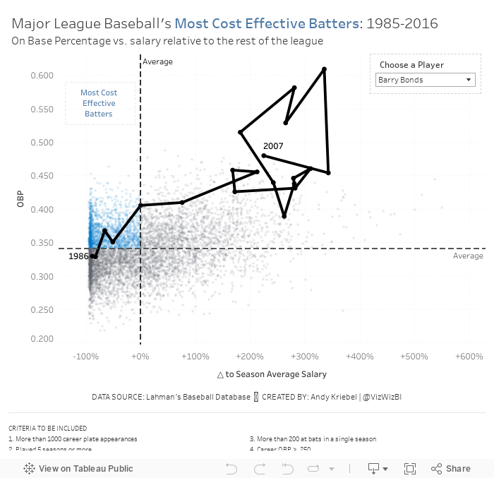
#MakeoverMonday: Major League Baseball's Most Cost Effective Players
baseball
,
connected scatterplot
,
cost effective
,
database
,
lahman
,
Makeover Monday
,
MLB
,
OBP
,
on base percentage
,
quadrant chart
,
salary
,
scatterplot
No comments


What works well?
- The title and subtitle explain what the viz is about.
- Dividing the viz into two sections by using different background colors on the scatter plots
- Consistent scales for the salaries across the charts for each section
- Using gridlines to help the audience understand the approximate values of each point
- Only labeling the type of stat once by putting the label between the players and teams charts
What could be improved?
- There's no data source listed.
- I have no idea why these players or team are highlighted; an explanation is needed. At first, I thought it was highlighting the most effective player/team, but it's not (at least that's what I see).
- The logos are meaningless for people that aren't familiar with the teams.
- What does the big logo on the upper right represent? Is that the author?
- The data should be filtered to players that meet certain criteria, like at bats in a season. This would then filter out many players near zero.
I liked the idea of using a scatter plot like the original, but I wanted to focus on a metric the better measures "effective". There are so many sophisticated metrics now in baseball. I didn't want to use any of those because they're hard for people to understand. I decided to use on base percentage which is the number of times a player reached base (H + BB + HBP) divided by at bats plus walks plus hit by pitch plus sacrifice flies (AB + BB + HBP + SF).
Why did I choose OBP? Ryan Kelley sums it up best in a post on Quora:
Outs are an extremely scarce resource in the economy of a baseball game, each team has 27 to use (in a 9-inning game) while trying to score as many runs as possible. Every time a batter makes an out therefore, the expected number of runs his team will produce will decrease (assume runs are also a limited resource for now).
A batter's job is to get on base--not make an out in other words. A batter fails to do his job when he makes an out, this failure percentage is 1 - OBP. The success percentage is OBP. If every batter had a perfect 100% OBP, their team would score an infinite amount of runs before every making an out.
Now, because you're talking about value specifically. OBP alone isn't effective in measuring value. You can make it a better indicator of value by giving it context. That context depends on what kind of value you're talking about.
You could tie OBP to a player's salary. This would give you an indicator of how value that batter was to his team in the context of a labor market. After all, baseball players are just employees of franchises in the end. Their jobs are to produce wins. A hitter's job is to produce wins via producing runs. Franchises make money by selling those wins to fans as entertainment.
Each team has a fixed amount of payroll to spend on wins, so the more payroll a batter's salary takes up, the less valuable he is to his team. A good way of illustrating a player's value would be OBP/$ of Salary.
Based on Ryan's explanation, I decided to use OBP as my proxy for batter effectiveness (y-axis). For the x-axis, I wanted to use salary for comparison. However, the data does not adjust salaries for inflation, so a salary in 1985 is not listed in 2016 value. Instead, I came up with a way to normalize the data across all of the seasons.
I created a calculation that compares a player's salary to that of the average salary of the entire league for each season. I made this a percent difference so that the data would then be normalized. Therefore, a player that was 10% above a 1985 salary would be comparable to players that was 10% above a 2016 salary.
Here are my calculations:
- Season average salary: { FIXED [Season] : AVG([Salary]) }
- △ to Season Average Salary: (AVG([Salary]) - SUM([Season avg Salary])) / SUM([Season avg Salary])
- First, I applied some filters to only include what I deemed "eligible" players. These are noted at the bottom of the viz.
- Now that I have the x-axis (salary variance from season average) and the y-axis (OBP), I created a scatter plot and added a point for each player for each season.
- I added reference lines for the average of each axis.
- The players on the upper left are the most cost efficient players. That led me to a quadrant chart, but I only wanted to highlight the most cost effective. I created a calculation to determine the points in that quadrant and place it on the color shelf.
- The problem now was that it was basically impossible to find a player in the viz. I thought about using a set action to drill in to a player, but that loses all of the context of the other players. Therefore, I create a parameter to allow the user to highlight a player and I show that players as a connected scatter plot.
SOME THINGS I FOUND
And here's my final product. I had never thought of combining a scatter plot and a connected scatter plot before. I'm quite pleased with how this turned out.
- Players tend to be more cost effective earlier in their careers. That makes sense since they are on rookie contracts for the first few years of the career.
- Once players sign their first big contract, they tend to either move to the upper right (high OBP, high relative salary) or the bottom right (low OBP, high relative salary).
- Some players can sustain that for the rest of of their careers, but that's rare. Typically it's the superstars that follow this pattern (like Barry Bonds or Chipper Jones).
- For many of the other players, as they approach the end of their career, they tend to move either to the lower right (high relative salary, low OBP) or the lower left (low relative salary, low OBP). Neither of these are particularly good for the team.
And here's my final product. I had never thought of combining a scatter plot and a connected scatter plot before. I'm quite pleased with how this turned out.
May 1, 2019
The UK's Most Popular Baby Names
Alteryx
,
baby names
,
data prep
,
flourish
,
office for national statistics
,
ONS
,
rank
,
UK
,
united kingdom
No comments

Sophie's Challenge
While Tableau is an amazing tool, when you use it all the time you can fall into data-viz-auto-pilot mode. You build the same kinds of charts; you construct similar kinds of dashboards; you fall back on the same formatting styles. While familiarity with tool, and a workflow, is a good thing, it also narrows your view of what’s possible.For today’s Dashboard Week challenge, I want you to step outside your data viz comfort zones and try building a viz using Flourish. Flourish is a free tool that lets your build interactive, responsive, and embeddable vizzes and data stories, all within the browser using your own data. Flourish is focused at the communication side of data viz (more than the data exploration side), and I’d like DS13 to really think about communication in today’s challenge.
Why Flourish? I really like their wide (and ever expanding) range of templates and interactivity (transitions, stories and ‘Talkies’ to name a few); also they are based in London – so why not viz-local?
Using any part (years, geographic locations, genders) of the England and Wales baby names data sets, I want DS13 to find and communicate one specific story from this data set.
Here are the rules for today, and what I’d like to see as output:
- They must work independently.
- Everything must be finished by 5pm.
- They must use Tableau and Alteryx for the data prep and exploration.
- The final viz must be made in Flourish.
My Approach
First, I had to get some data. I decided to download the data from the ONS for 1996-2016 because it was in a relatively decent format.Next, I opened the "Plotting Competitors" example because I loved the animation. The great thing about Flourish is you can immediate use the template. All you need to do is upload your own data, assign the columns, and you're done!
This meant I had to do some data prep in Alteryx to get it in the correct shape. I needed the years across the view and the number of births for each name and gender. Then I filtered both the boys and girls to the 25 most common names, giving me 50 names in total.
I absolutely LOVED playing with Flourish and will definitely use it in an upcoming Makeover Monday.
Check it out! The animations are so so good! There were straight line and curved line options. I went for the curves. Enjoy!
Subscribe to:
Posts
(
Atom
)


