May 17, 2021
#MakeoverMonday Week 20 - Humans vs Animals

WatchMeViz
Visualization
March 27, 2017
Makeover Monday: The Secret of Success

Andy Cotgreave messaged Eva and me about this particular viz and found a great article that does an excellent in-depth review of this particular piece. Reading the article helped reassure the thoughts that I've had about this chart over the years.
What works well?
- Engaging design
- Clear labels on the values
- Legend matches the shape of each amoeba
- Everything is scaled in proportion
- Good color choices
- Nice big title
- The subtitle is very offensive. It sure seems this survey was conducted by some extreme right-wing group.
- The overlapping colors make it hard to follow the pattern.
- Radar charts are very hard for making comparisons across categories.
- The radars are curved to make the segments appear to take up more space.
- Unnecessary icons
May 17, 2016
Tableau Tip Tuesday: How to Create Monthly Radar Charts

In this week’s Tableau Tip Tuesday, I show you how to create radar charts that are based on monthly data. That is, the months go around an imaginery circle like a clock. Thanks to Jonathan Trajkovic for this great explanation and to Ed Hawkins for the inspiration.
May 15, 2016
Makeover Monday: How warm is Earth becoming?

There was a lot of chatter on Twitter last week about this terrific visualisation by Ed Hawkins:
Spiralling global temperatures from 1850-2016 (full animation) https://t.co/YETC5HkmTr pic.twitter.com/Ypci717AHq
— Ed Hawkins (@ed_hawkins) May 9, 2016
The beauty of this visualisation is in the animation. However, without the animation, it kind of fails to tell the story. Let’s dig a bit deeper.
What works well?
- There is a clear title.
- The background circles provide helpful context.
- Including the month labels makes it easier to understand what you’re seeing.
- The year in the middle helps tell the story.
- The animation is compelling.
- It has a nice color scheme that works well on a black background.
What could be improved?
- While the title is clear, it could be more eye-catching, like a news headline.
- If you see this as a static image, you lose the sense of change.
- You can’t compare any time periods. All you know is 2016 is the warmest.
- There’s no explanation about what the numbers represent. Though I do see in the Twitter post a link to additional information.
- The color scale has nothing to do with the temperature change, which I assumed it did until I read hte additional information. The colors actually represent the years. That doesn’t add much value. I think coloring by the temperature change would be more impactful.
So, this data set is actually incredibly simple. All we have is one record per month, the temperature, and the confidence intervals.
The first thing I wanted to do was rebuild the radial chart. This wasn’t nearly as easy as I thought. This post by Jonathan Trajkovic was very helpful, but it wasn’t designed for months. I’ll record how I did made it for a future Tableau Tip Tuesday.
 |
| Click the image for the interactive version |
This radial chart is basically the same as the original, however I can’t make it “play”on Tableau Public and I also changed the color to be the median temperature difference. Really, I only built this to see if I could. It’s not any more useful than the original.
Next, I took the radial chart and flattened it out.
 |
| Click the image for the interactive version |
This doesn’t make the understanding all that much easier because I can’t tell which years are which. Maybe I should switch the color legend back to years?
 |
| Click the image for the interactive version |
Oh wow! What a difference! Now I can easily see the distinction between the older and more recent years. I think this is much, much better than the original, especially in static format. I wanted to keep iterating though.
Whenever I’m working with time-based data, I like to build either calendar heatmaps or heatmaps by year and month. Here’s what this data set looks like as a heatmap:
 |
| Click the image for the interactive version |
The heatmap makes the series of lines even easier to understand. It’s super easy to see the gradual temperature change over time. This is pretty compelling, yet I wanted to keep going. Was there a better way to tell the story?
Next I looked at the 10-year average, that is, a 120 month moving average of the median temperature change. I then overlaid the confidence intervals.
 |
| Click the image for the interactive version |
Lastly, I took the 10-year moving average view and replaced the monthly confidence intervals for the monthly values while keeping the overall 10-year average. This is my submission for Makeover Monday. In this view, I like how I can see the drastic monthly fluctuations but still have the overall context. Including a reference line at zero helps emphasize the dramatic change since about 1984.
I also included a strip plot under the graph that shows the average median temperature difference for the entire year. This brings back a bit of the heatmap view above.
In the end, another fun week with a simple data set that provides lots and lots of options. Which one do you like best?
UPDATE: This week has been a fascinating exercise in iterating. That’s the beauty of Tableau. I can get another idea and build it quickly. After seeing some of the submission for this week, I thought a jitter plot might work well. Thoughts?
 |
| Click the image for the interactive version |
June 4, 2015
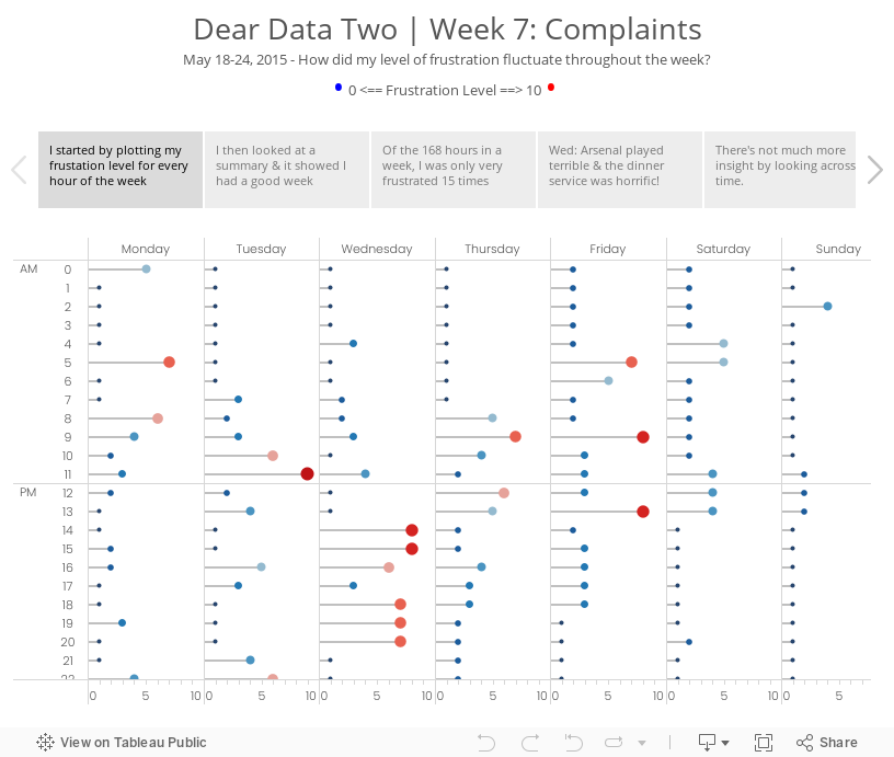
Dear Data Two | Week 7: Complaints

For week 3 Jeffrey sent me a donut chart by accident (so he says…) and while I was thinking about my ideas for this week, I started connecting some data points with lines and ended up with a radar chart. (See the draft version in the story points.) It’s funny how he and I both have gone against what we would consider best practices. What does that mean??
I decided to go with a clock them this week and split the data up between morning and afternoon. From there, I plotted each day going outward from the centre for that hour. For example, at 12am, Monday is closest to the middle and Sunday is farthest from the middle. This helped me see which hours were cumulatively the most frustrating for me for the week. Each dot is separated by the frustration level. If the frustration level was three, then the dot would be 6mm from the previous dot. I then sized the dots by the frustration level so as to double encode the values.
It’s no surprise that my sleeping hours were generally the least frustrating, except for 5am when jetlag kicked in. Overall, 9am was my worst hour in the morning and 1pm was the worst in the afternoon. The story points viz below goes into more of the explanations.
April 29, 2013
Artic Sea Ice Volume: A Radar Graph vs. Line Graphs
UPDATE (May 2, 2013): I have removed 2013 from all charts.
I posted an article on my Facebook page the other day asking if this radar graphs about artic sea ice volume works. The comments were mixed.

I think this radar graph is merely ok. Radar graphs, in general, are hard to read because relationships and trends are not easily discerned. Some of the issues I see with this graph include:
- It’s difficult to see the entire pattern over time. I see the pattern is spiraling in, but does it change year by year. Ask yourself this: How does 1999 compare with 2004? It takes a lot of work.
- It’s very hard to follow the ice volume labels around the chart. I bet you found this as well in the example above.
- The author only included September. Why? The data is available by day. Get the data here.
- Are there any seasonal patterns? You can’t answer this question.
I created a couple of different views for your consideration in Tableau. You can download the workbook here.

In my version, I’ve addressed all of the problems I mentioned above.
- In the upper left graph, you can easily see that the artic sea ice volume is trending down.
- The upper right chart allows you to see two things:
- The seasonal patterns
- Comparisons by year: The comparisons across years can be see because the years get darker as the data gets closer to 2013. You can see the lines get darker as you look down the graph.
- The Daily Volume graph makes the cyclical patterns much, much clearer.
How would you visualize this data? Do you agree that these line graphs work better than the radar graph?